Total Solar Eclipse
2024 April 8
Overview
North America’s second total eclipse of the past seven years comes at a very different season than that in 2017. April is a month of transition across the continent, with winter storms gradually giving way to the convective buildups of spring and summer. In Mexico, the winter dry season is in its last month before the summer rains begin. Over the United States, southern parts of the track are already well into the thunderstorm season, while to the north, spring storms and occasional snowfalls still hint of the departing winter. In Maritime Canada, the last of the winter snow has yet to melt and fresh snowfalls are a threat with every weather system. Finding that magical viewing spot will be much more demanding than seven years earlier.
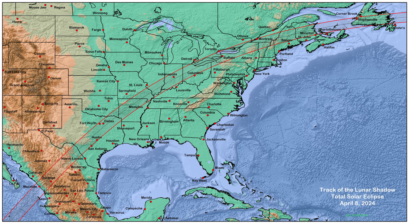
In the 2017 eclipse, the rugged terrain of the western mountains had a large influence on the formation of clouds. Locations in the lee of high terrain tend to be sunnier—sometimes considerably sunnier—than those on the windward side. In this eclipse, mountain terrain is only important in Mexico, where much of the track is sandwiched between the Sierra Madre Occidental mountains along the Pacific Coast and the Sierra Madre Oriental along the Gulf of Mexico (Figure 1).
From Texas to the Great Lakes, the track moves across the low topography of the Great Plains and the Mississippi Valley where terrain and cloud-cover variations are muted. Only after reaching the Middle Atlantic States south of Lake Erie does the southern side of the Moon’s path cross the rugged topography of the northern Appalachian Mountains where some advantage might be gained by hiding behind a topographic barrier. Unfortunately, the spring season and the location of the storm tracks through this area superimposes the benefits given by the terrain onto a very cloudy climatology, giving limited relief to eclipse travellers. Somewhat surprisingly, it is the presence of water—the Great Lakes and the Gulf of St Lawrence—that has the biggest impact on cloudiness.
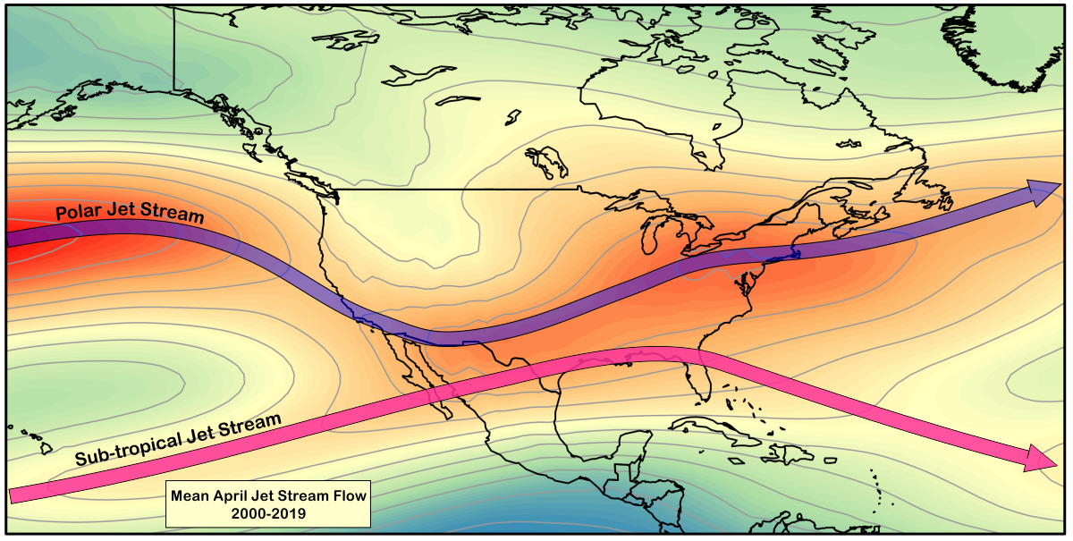
The chart of average April sea-level pressure shown in Figure 2 sets the stage for this discussion of eclipse weather. Two high-pressure systems straddle the North American continent, one northeast of Hawaii in the Pacific, the other between Bermuda and the Azores in the Atlantic. In April, these anticyclones are beginning to strengthen from their winter minimums, though they have only a limited effect on eclipse-day weather . Over the continent, a poorly organized surface low lies along the eastern foothills of the Rocky Mountains with a low-pressure trough extending across the Great Lakes and Newfoundland to join up with a deep low near Iceland.
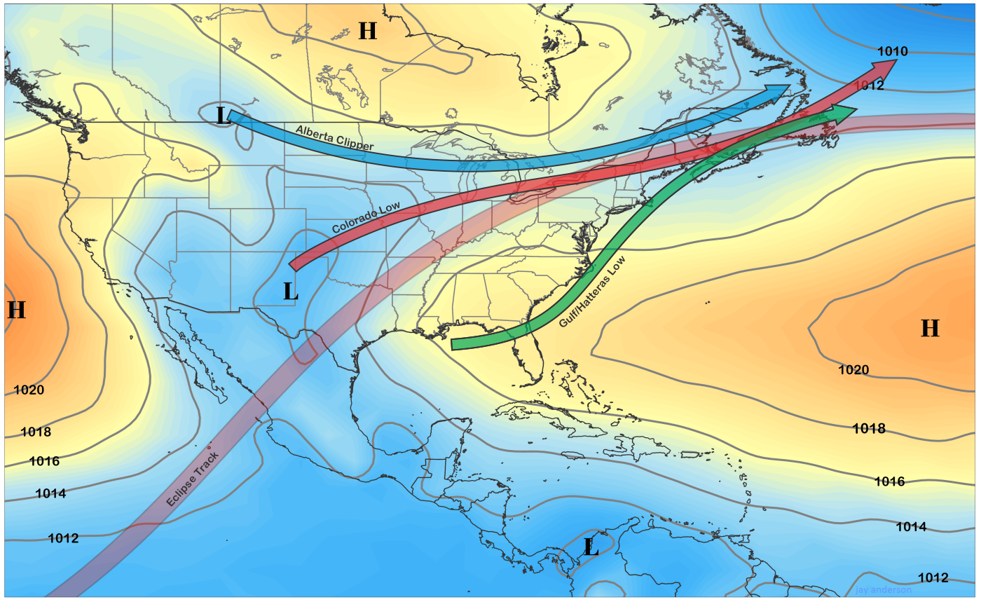
The low-pressure centres and their extended troughs roughly mark April’s major storm tracks across the continent. In Figure 2, we see three of the most important tracks: the Alberta Clipper, the Colorado Low, and the Hatteras Low (which may be called a Gulf Low at its start and a Nor’easter in New England). The tracks shown in Figure 2 are schematic, as the actual paths can be highly variable. These storms are large systems with extensive cloud shields that can almost entirely obscure the U.S. and Canadian portions of the track if one happens to lie in the wrong position on eclipse day.
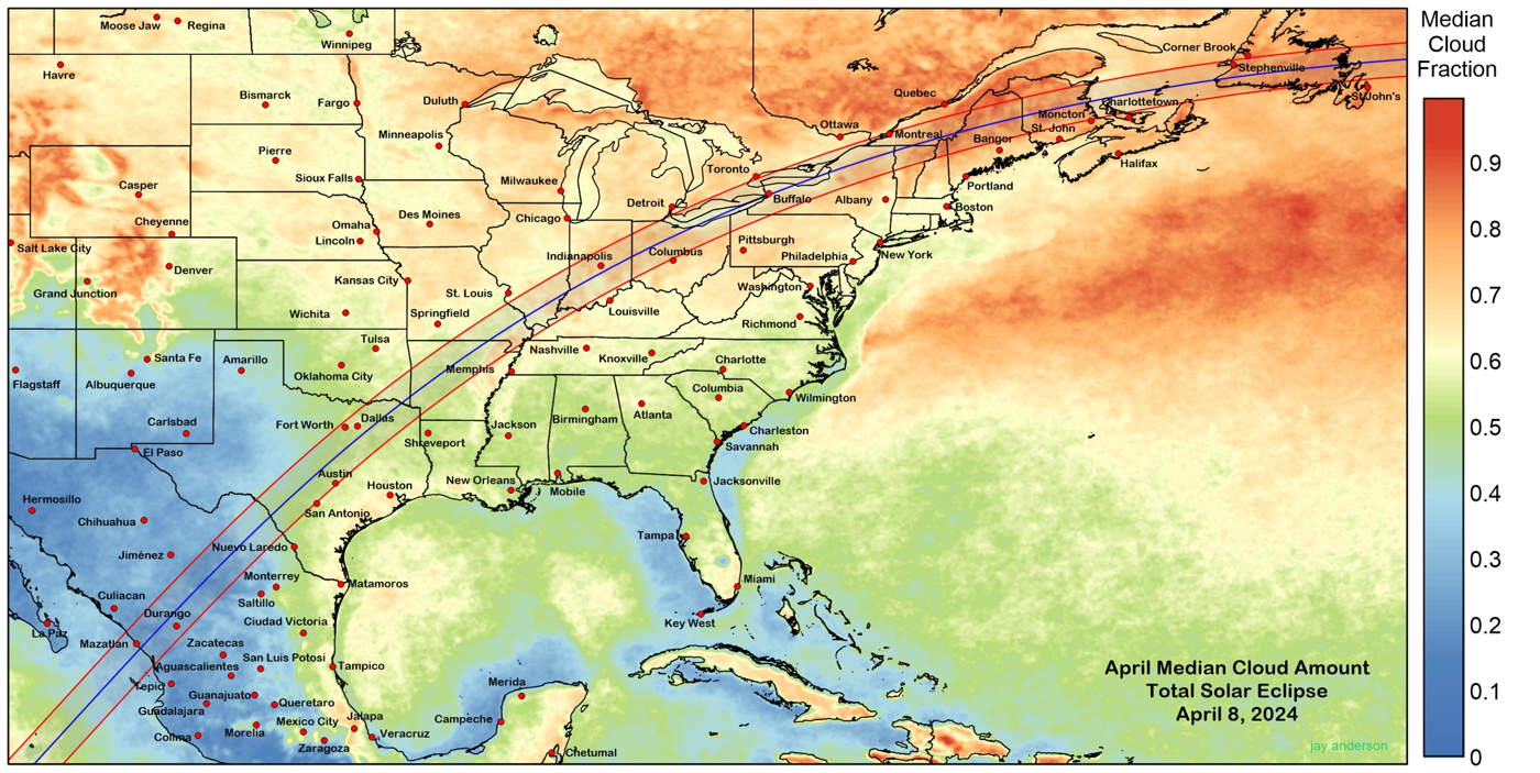
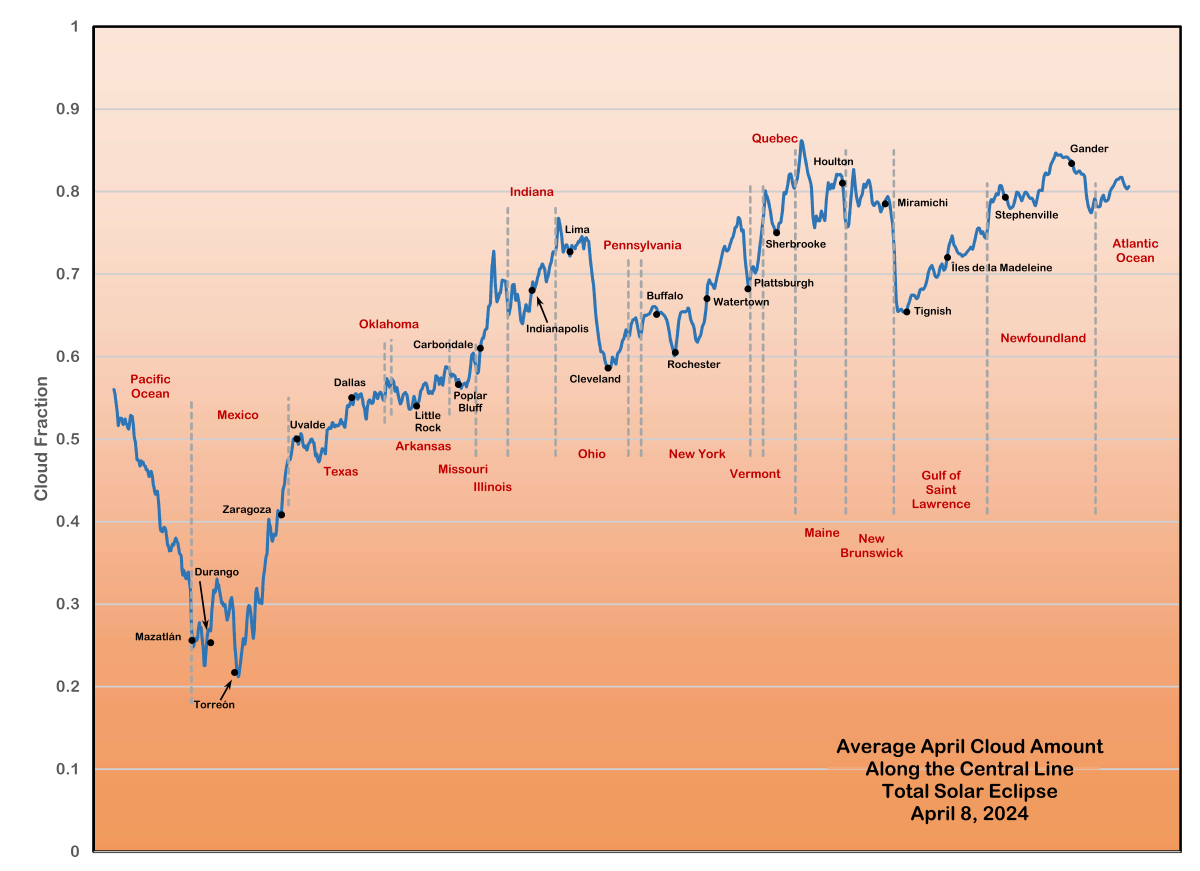
Given the scenario described above, it is no surprise that the frequency of cloudy weather increases steadily along the south-to-north track of the lunar shadow (Figure 3). Across almost all of Mexico, median monthly cloudiness as measured from satellite barely reaches 40 percent. This percentage increases rapidly as the shadow path approaches the Texas border, and increases abruptly again in Missouri, climbing to 75 percent in Indiana and Ohio, after which it zig-zags up and down between 65 and 85 percent until it leaves the North American continent (Figure 4). Even in the cloudiest regions, however, there are hopeful signs: abrupt drops in cloudiness along the Great Lakes and across the Gulf of St Lawrence offer the prospect of some sunnier refuges for eclipse seekers on April 8. In this eclipse, much more than in the fair-weather climate of 2017, advance preparation and attention to weather forecasts may prove to be critical for a view of the masked sun.
The trend in cloudiness revealed by the satellite data is mirrored by measurements from the ground. Precipitation amounts and precipitation days follow the upward trend of the cloud frequency and the amount of sunshine trends downward.
The Impact of El Niño
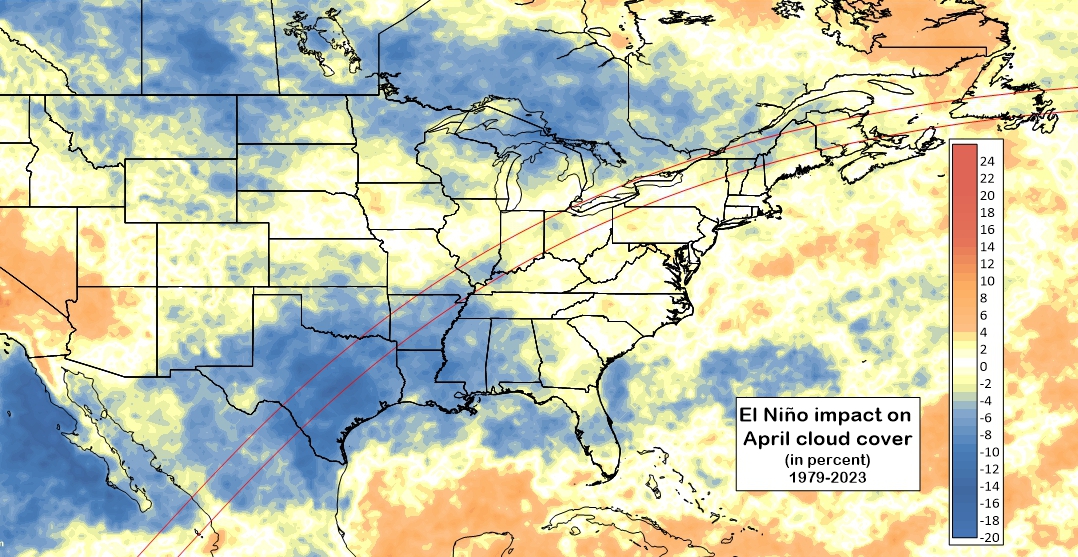
During the late summer and autumn of 2023, temperatures along the equator in the upper levels of the equatorial Pacific Ocean began to rise and a few months later, a strong El Niño event became established. Because of the amount of heat contained in those waters, significant meteorological changes occur in parts of the global weather, particularly in North America. A more complete description of the phenomenon can be found here.
For eclipse watchers, the primary question is whether El Niño will affect the cloud-cover climatology along the shadow track. By April, El Niño should be fading away if it follows its normal pattern, but effects on the North American weather can continue for a few months longer into spring. To answer the question, satellite measurements of April cloud cover from 1979 to 2023 were gathered and sorted into years following neutral ocean temperatures (aka “normal”) and years following an El Niño. Monthly averages for each category were calculated; April neutral-year cloud amounts were subtracted from April El Niño-year amounts.
Figure 4a shows the results of this exercise. Blue tones denote regions with lower average cloud amounts in an April following an El Niño winter; white and pale yellow tones show those parts of the continent with little or no impact from El Niño; and orange tones suggest regions with higher April cloud cover.
It is apparent that Texas will be most likely to benefit from the current El Niño with cloud amounts as much as 15% lower (north of San Antonio) than in neutral years. The full amount of the difference cannot be completely applied to Figure 3 (i.e. you can’t just subtract 15% from the map) since the data for Figure 3 already includes El Niño years in its construction.
Mexico
By the time that the lunar shadow reaches the coast of Mexico, it is already nearly 7,000 km and 90 minutes old, having touched down at dawn in the mid-Pacific, 65 km north of Penrhyn Island (Tongariva) in the northern Cook Islands. From there, it’s a long haul across the ocean until the shadow’s introduction to Mexico, at Isla Socorro, a small volcanic outcrop lying 680 km west of the mainland, and the first of a half-dozen small islands before the continent. The marine environment surrounding the islands guarantees a relatively high cloud cover in offshore Mexico, but cloudiness declines rapidly as the eclipse track approaches the mainland beaches near Mazatlán.
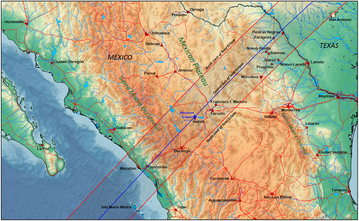
The Mexican coast presents an abrupt mountain barrier to the sea (Figure 5) and so the eclipse path has only a narrow 25 km coastal plain to cross before beginning to rise over the Sierra Madre Occidental; within 100 km of the coast, the terrain has risen to over 2600 m. The Occidentals are a rugged range with 500-m deep valley basins cutting into the mountain topography. Once across the Sierra, near Durango, the Moon’s path enters onto the Mexican Plateau, a rough inland mesa consisting of desert plains interspersed with low mountain ridges. North of Torreón, the shadow track passes over the Bolsón de Mapimí, a large ill-defined inland basin that stretches north to Presidio on the U.S. border.
The Bolsón provides only a brief respite from mountain topography, for barely 60 km beyond Torreón, the track begins the ascent of the Sierra Madre Oriental, the eastern counterpart to the Occidental range along the Pacific coast. Though there are individual peaks in the Sierra Madre Oriental that are as high as those in the Occidentals, in general, the Oriental is not as rugged and is cut by many valley openings that are exposed to the lower elevations of the Gulf Coastal Plains. The eclipse track eases out onto the coastal plains beyond Monclova, and elevations drop abruptly from about 1800 m to 400 m and then more gradually to 200 m as it reaches the Texas border and the Rio Bravo/Rio Grande floodplain.
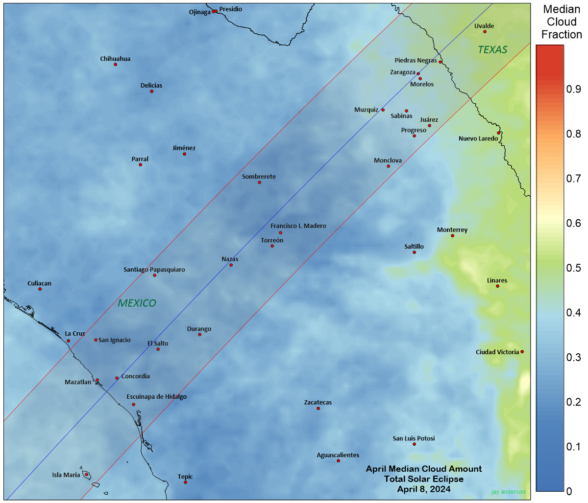
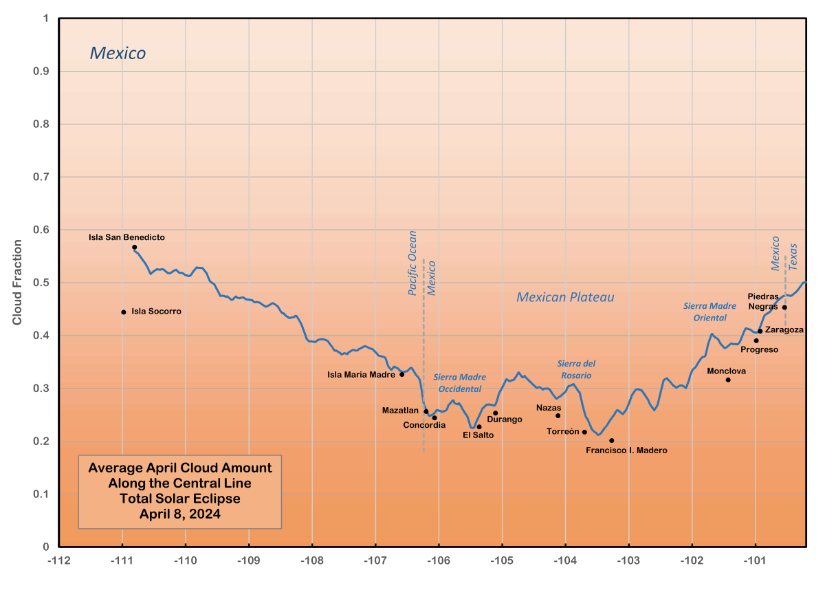
The dry-season climatology of Northern Mexico in April promises a generous probability of sunny weather for the eclipse (Figure 6) though the measurements of cloud cover from all sources may be underestimated because of the frequent presence of thin cirrus-level clouds. In the satellite measurements, centreline cloudiness barely budges from the 25 to 35 percent range from Mazatlán to the start of the Sierra Madre Oriental—a very generous climatology as eclipse travel goes (Figure 7). Only when the track reaches the east side of the Orientals and descends onto the Gulf Plains does the cloud cover rise, from around 30 percent at Monclova to near 50 percent at Piedras Negras and the U.S. border.
Though Mexico has a very sunny climate, we cannot lose sight of the fact that approximately one-quarter to one-third of skies are cloudy enough to have an impact on viewing the eclipse. The main sources of cloudy weather can be chosen from an eclectic mixture:
- High-level cloud carried across the region by the sub-tropical jet stream
- Cold fronts that drop southward from the U.S. Great Plains onto the Bolsón de Mapimí
- Convective clouds—especially thunderstorms— that form along the eastern slopes of the Sierra Madre Occidental and Oriental
- Low cloud that moves inland from the Gulf of Mexico onto the Rio Grande floodplain and the Gulf Coastal Plain
The sub-tropical jet stream (Figure 8) is a major annoyance for astronomers in Mexico, Arizona, New Mexico, and Texas, carrying extensive sheets of high-level cloud through the region and curtailing night-time imaging. In April, the jet is always somewhere in the neighbourhood, flowing from southwest to northeast, and may impact the eclipse track anywhere from Northern Texas to Central Mexico. If the flow of wind aloft is relatively weak, the jet stream may carry only thin wisps of cloud; stronger jets will bring increasingly opaque cloud cover, typically at cirrus and high mid-cloud levels and can be a major problem for eclipse visibility. These high-level clouds pose the greatest threat to eclipse-day weather in Mexico. They are not captured very well in either the surface-based sunshine statistics or the satellite cloud measurements as they are usually semi-transparent, giving an illusion of sunshine when the sky has a veil of cloud. On the other hand, their semi-opaque nature should allow the eclipse to be seen, though more-or-less hazily.
The energy contained in the upper winds may interact with lower levels to intensify a cold front or promote the development of thunderstorms along the slopes of the Sierra Madre Occidental.
Cold fronts that swing down into Mexico from Texas and New Mexico are also a big problem; they can bring extensive areas of cloud and a tendency to form deep convective buildups. These fronts can penetrate far into Mexico, certainly across the eclipse track, though they are much more intrusive on the inland east side of the Sierra Madre Occidental than on the Pacific side. As with all cold fronts, they come with many levels of intensity. Some bring clumpy mid- and high-level clouds. Others, more active, bring large cloud shields with embedded showers and thundershowers.
On sunny but unstable days, convective clouds may form on the mountain ridges and on east-facing slopes, taking advantage of the absorption of sunlight by dark, forested hilltops that raises temperatures and initiate the growth of showers and thundershowers. The largest of these convective storms send cloudy debris across the Mexican Plateau to plague eclipse seekers. These buildups and their debris cloud are probably the explanation for the higher cloudiness over the plateau between Durango and Torreón in the graph of Figure 7. Finding sunny weather can be challenging in a highly convective atmosphere, but the road from Durango to Torreón, which offers a route that parallels the central line for 250 km, might provide a means to escape into sunshine. Fortunately, thunderstorms are more likely to build after the passage of the lunar shadow.
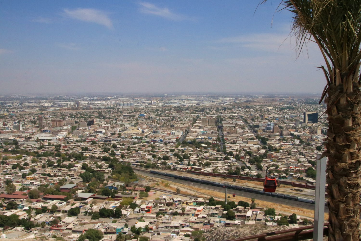
Torreón itself lies in the shelter of a small range of hills that tower 800 m above the city centre and which are capable of generating their own convective showers and thundershowers, usually late in the day when the ground has warmed to its maximum. One of the peaks hosts Cerro de las Noas, a public overlook that contains the Cristo de las Noas sculpture and a small observatory owned by Planetarium Torreón. The site can be reached by cable car from the midst of the city and would provide an all-encompassing site from which to view the eclipse at a location close to its maximum point.
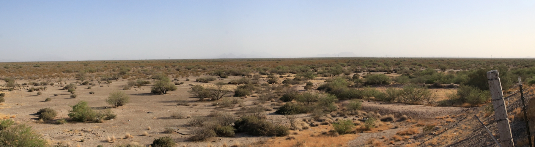
The Bolsón de Mapimí, north of Torreón, is a dusty place, with many dust devils to load the atmosphere with aerosols on a typical sunny day. The low-level dust will have a minimal impact on eclipse visibility, as the Sun is over 70 degrees high, but will mask the horizon in wide-angle photography.
On the narrow coastal strip around Mazatlán, convective clouds are uncommon and southward-sweeping cold fronts make little impact: the frontal cloud and moisture are blocked by the heights of the Sierra Madre Occidental. Most cloud on the Pacific side of the mountains comes from jet stream cirrus and mid-level cloud, similar to farther inland. While the Mazatlán coast doesn’t have the greatest sunshine along the eclipse track, it’s only 3 to 5 percent cloudier than measured at Durango and Torreón from the satellite.
Morning fog or low stratus clouds that form offshore overnight and come ashore along the coast may also be a problem, as they tend to be drawn inland as the sun rises. The fog or stratus will burn off or thin later in the day, but that may not happen before eclipse time and there is a risk that the fog will re-form as the air cools ahead of totality. The only reliable way to escape the fog is to move away from the coast and uphill. Fog will reach inland until it encounters altitudes of 100 or 200 m, but stratus clouds can reach much farther, as far as Copala, a distance of 50 km from the coast and 500 m in altitude. This higher ground can be reached using Highways 40 and 400, south of Mazatlán, which run alongside the eclipse centre line for more than 60 km. That’s more than enough distance to escape fog and low stratus and find an open spot to view an almost-overhead sun. Large groups may have a problem to find a spot to spread out, as the inland is heavily treed. Google StreetView will help to find a location.
The least promising eclipse-watching sites in Mexico come after the track has passed the Sierra Madre Oriental and moved onto the Gulf Coastal Plains as it approaches the Texas border. Satellite photographs show that low-level moisture from the Gulf of Mexico often floods across the coastal plain, moving northwestward toward the eclipse track beyond Nuevo Laredo. On most days, it doesn’t quite make it to the track and as the day warms, the cloud tends to retreat a bit, back toward the coast. Southeast of Monterrey, the cloud piles up against the steeper parts of the Orientals, but farther northwest, the mountain range becomes quite broken up, and the coastal cloud is sometimes able to worm it way west to Monclova, though that is uncommon. The moisture feeds the occasional thunderstorms that pop up in the border region. The presence of the coastal moisture and the greater exposure to cold fronts dropping southward from Texas is the main reason for the 15-percent growth in cloudiness as the eclipse track leaves the Mexican Plateau and reaches the U.S. border.
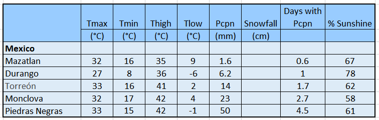
Temperatures are pleasant for the most part in Mexico (Table 1), though the overnight lows can approach the freezing point on the Mexican Plateau. Sunshine measurements are generous, especially when we realize that the measuring instruments do not respond in the early morning or evening when the Sun is low, even if skies are clear, and so have a bias toward low sunshine percentages.
Texas to Missouri
When the Moon’s shadow crosses the Rio Grande and moves into the United States, it traverses the floodplain of the Rio Grande River where elevations are between 200 and 300 m above sea level (Figure 9). Immediately afterward, the shadow meets the Balcones Escarpment and rises up onto the Edwards Plateau, an increase of about 400 m in elevation. After passing San Antonio and Austin, the track descends onto the Gulf Coastal Plain and later, the Mississippi floodplain, passing Dallas and Fort Worth on its way to the Oklahoma and Arkansas borders.
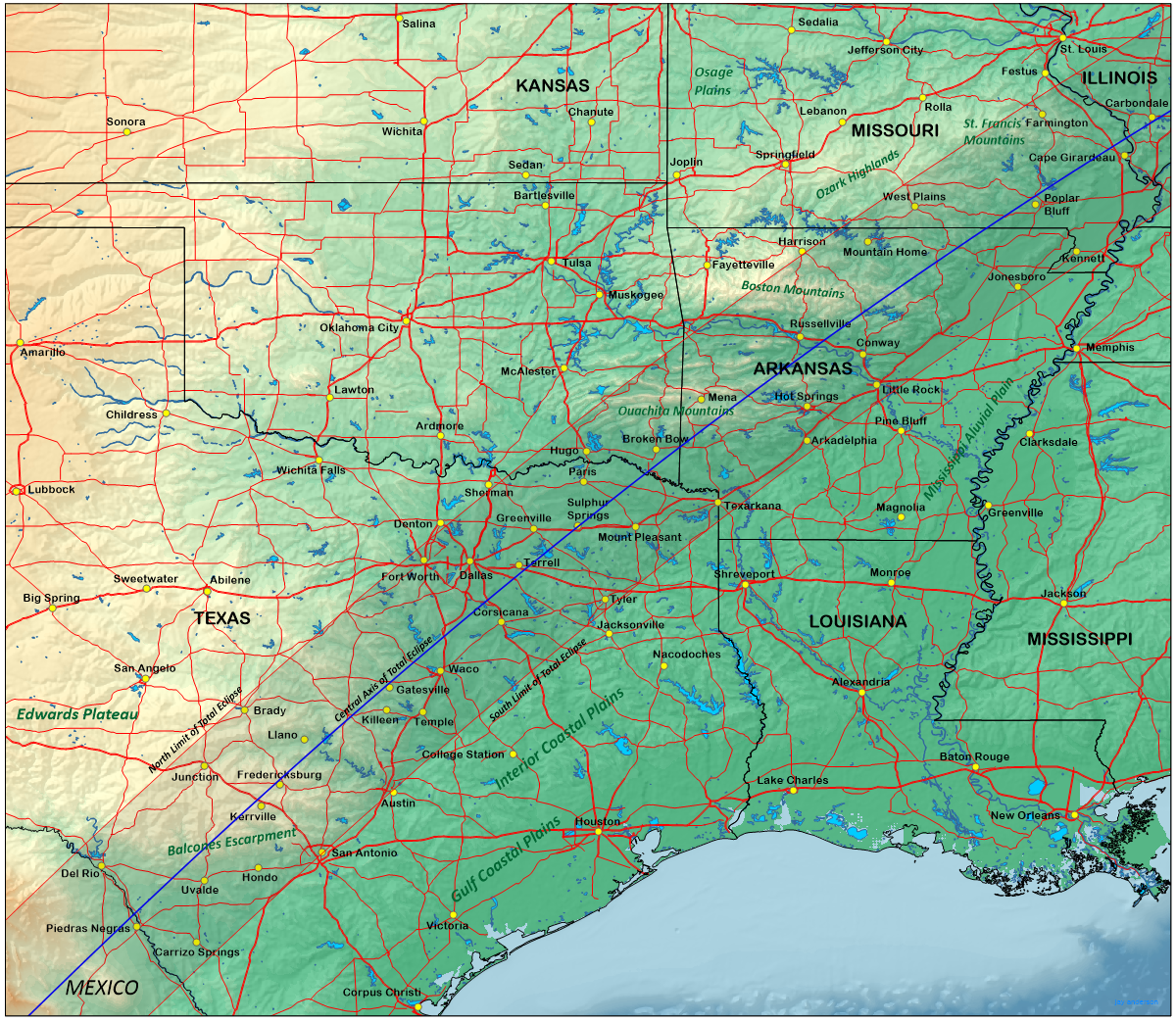
Through Oklahoma, Arkansas, and Missouri, the topography along the eclipse track is an up-and-down roller coaster with several small mountain chains interspersed with flatter plateaus (Figure 9). The Ouachita Mountains straddle the eclipse track across the Oklahoma-Arkansas border and farther along, the Boston Mountains underlie the north side of the shadow’s path beyond Russellville, Arkansas. The track settles onto the Ozark Plateau as it moves into Missouri, and later, just touches the St Francis Mountains on its north side as it reaches the Missouri River. All along the Oklahoma to Missouri part of the track, there is lower ground to the southeast side of the path (the Mississippi Alluvial Plain) and higher ground to the northwest.
As we look along the graph of centreline cloudiness for this region (Figure 10), we see a modest increase in cloud cover from the Mexican border to the Missouri River. Most of the rise takes place in Texas where the eclipse path moves from dry-season desert climatology into mid-latitude springtime weather. April is a month that has both a summer and a winter personality, sometimes with convective thunderstorms (including severe weather) and at other times, cold-season low-pressure storm systems.
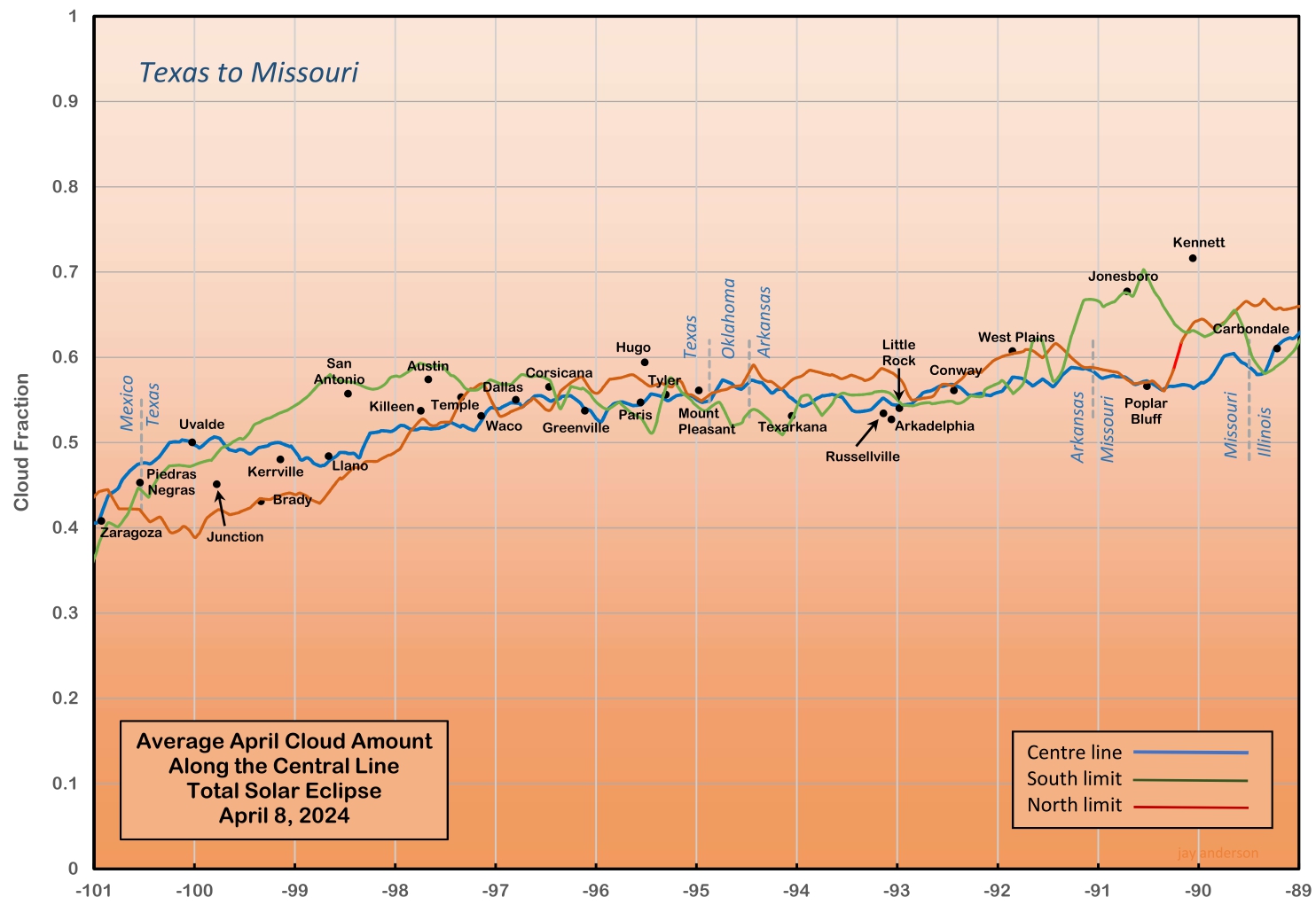
One of the more interesting aspects of the cloud cover over this part of the track is the occasional wide variation of cloudiness across the shadow path. The south limit near San Antonio, exposed to the frequent intrusions of Gulf Coast moisture and low cloud, is nearly 20 percent cloudier in April than the north limit near Junction. It is only after the track passes Dallas that cloud cover becomes more uniform across the path.
A large part of the difference in cloudiness in southern Texas can be explained by the rising terrain in the Hill Country as the Gulf Coastal Plain rises to the Edwards Plateau. Low stratus clouds are often not deep enough to overcome the 500 m rise from San Antonio toward Junction, though on rare occasions they may spread into New Mexico. There are other terrain-induced cloud discontinuities across the track, particularly near the Arkansas-Missouri border (Figures 10 and 11),
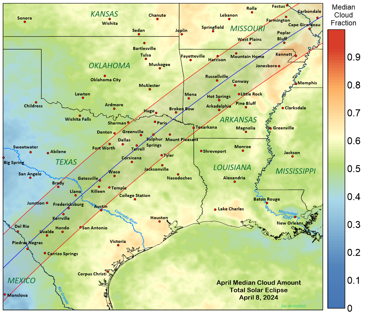
Across Texas, the north side of the track has a notably sunnier April climate than the south. The best of Texas weather prospects—in fact, the best prospects in the United States and Canada—lies on the Edwards Plateau, where median cloud amounts are as much as 15 percent lower than those south of the centre line on the Coastal Plain. We can be even more specific: according to the satellite data, the best climatological prospects lie between Junction and Brady, both in Texas. Brady is perilously close to the north limit but Junction, 28 km inside the track, has an eclipse duration of 3m 7s, generous, but significantly shorter than the 4m 26s at the centreline near Kerrville. Satellite measurements show a median April cloud fraction of 39 percent (0.39 on the map) in the area. Junction is connected with Kerrville and San Antonio by Interstate 10, which provides a convenient cross-track route to better weather from those locations if movement is necessary on eclipse day. Don’t leave it to the last minute—the 2017 eclipse taught us that even Interstates will come to a halt when the eclipse is imminent!
Another good eclipse-viewing spot is one tucked up against the Mexican border where cloud amounts are only fractionally greater than at Junction, generally between 40 and 45 percent. The town of Eagle Pass, opposite Piedras Negras, Mexico, which lies close to the umbral axis, may provide a convenient home base for those who wish to remain in the United States. Movement across or along track from Eagle Pass can be accomplished along State Highway 277, which leads to Del Rio to the north and Carrizo Springs to the southeast. Figure 10’s graph also points to a location near Llano as a low-cloud site for those who wish to immerse themselves right in the middle of the umbral shadow.
Past Llano, cloud amounts climb slowly along the shadow path, rising from 47 to 56 percent along the eclipse centreline. Mottled greenish colours in Figure 11 reflect small pockets of higher and lower cloudiness, but these are relatively insignificant. Through Oklahoma, Arkansas, and most of Missouri, cloud cover along the track axis varies through a 5 percent range, between 54 and 59. It is not until the eclipse shadow is almost in Illinois that cloud amount reaches above 60 percent.
When we look off of the centre line, however, the situation is not so simple. Beyond Little Rock, Arkansas, the south side of the shadow moves over the lowlands of the Mississippi Alluvial Plain (Figure 9) while the north side rests on the higher terrain of the Boston Mountains and the Ozark Plateau. An eclipse-track cross-section north of Little Rock would show an elevation of 650 m above sea level in the Boston Mountains near the north limit, and an elevation of only 70 m at the south limit, on the Mississippi Plain.
The boundary between cloudy lowlands and sunnier heights is quite abrupt, especially in Missouri, where the transition in cloudiness shows as a sharp change from orange to green tones in Figure 11. The low-lying floodplain of the Mississippi River is a “reservoir” of atmospheric moisture that hides under heavy stratocumulus layers or blossoms with convective clouds on unstable April days while the hills to the west remain in sunshine. It’s not an everyday event, but happens often enough, especially just after larger systems have passed by to the east, that the cloud statistics are strongly affected. Jonesboro and Kennett, which lie on the floodplain, have 10 to 15 percent higher April cloud amounts than stations on the north side of the track. From Little Rock northeastward, it’s probably best to stay north of the centreline and head for the high ground on the Ozark Plateau unless the weather forecast promises a sunny day right across the track.
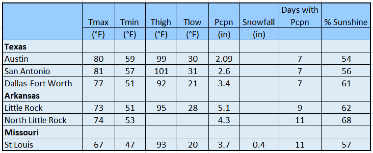
For the most part, average afternoon temperatures are very pleasant across the Texas to Missouri portion of the eclipse track (Table 2), though record highs run into the low 90s (33°C) and record lows can drop as low as the freezing point (or lower, in Missouri). In Texas, about 7 days of the month report rain; in Arkansas and Missouri, rain comes on about 10 days. Snowfall is largely unknown south of Missouri in April. We include the station statistics showing the percentage of sunny hours compared to the number of hours from sunrise to sunset in Table 2, but these are old data, not updated since the mid-1990s for the most part, and have observational biases that limit their usefulness.
A note about severe thunderstorms
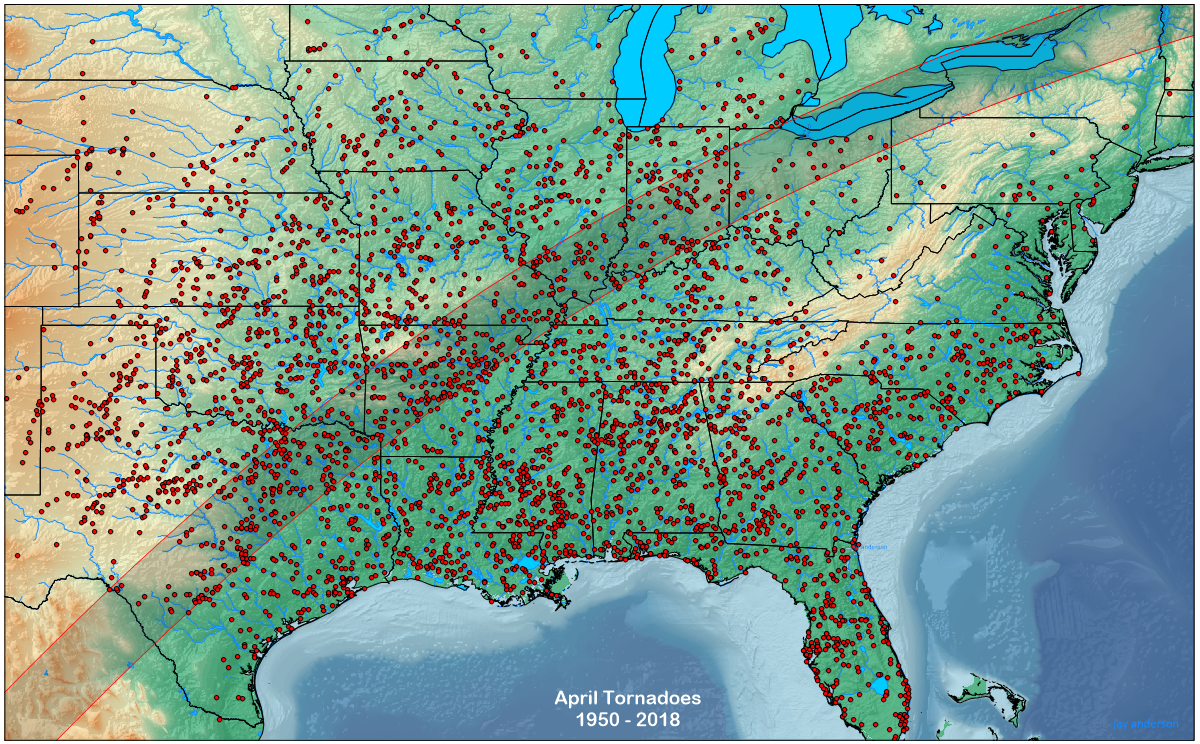
Until the eclipse track passes Ohio, typical April weather can include a threat of severe thunderstorms, including tornadoes, though they usually hold off until later in the afternoon, after the shadow passage. Figure 12 shows the locations of all April tornadoes reported to the National Weather Service in the 69 years from 1950 to 2018. Without putting too fine a point on it (as Dickens would say), the eclipse track passes through a fairly dense concentration of reports over Texas, Arkansas, and Illinois. Since tornadoes are fed by moisture advecting from the Gulf of Mexico, there are fewer of them on the Edwards Plateau in Texas where the elevation of the land limits the penetration of the ground-hugging, high-humidity air. Figure 12 cuts off at the U.S-Mexico border, but April thunderstorms are also a frequent event in Mexico, especially over the Rio Grande floodplain.
Tornadoes are a pretty localized event, but the systems that spawn them also dump a large mass of mid- and high-level cloud into the atmosphere and the extent and opacity of those clouds is not always captured by the models that predict the weather. The location and initiation time of those storms is also a bit dicey, and while they can be predicted in general, their rapid formation can bring on a late and unavoidable surprise. If you can find an accomplished storm chaser to join your eclipse party, you will find them a valuable source of information and reassurance.
I have a vision of a horde of eclipse chasers running out from under the cloud cover created by a severe storm while an equal number of storm chasers rush in the opposite direction to see what might transpire within the storms.
Illinois to Ohio and Southwestern Ontario
As the eclipse track reaches Illinois, it moves into the path of the mid-latitude spring storms: the Alberta Clipper, the Colorado Low, and their various cousins. These are names given to the more intense low-pressure systems, but there are many weaker ones that bring a day or two of cloud and then depart eastward, leaving only a few centimetres of snow or millimetres of rain. At this latitude, they are a regular spring event, probably every three or four days. Storms approaching from the west will first spread a thickening veil of cloud across the eclipse track and then eventually bring precipitation as they come closer and thicken. At the approach, warm southerly winds will dictate that rain is most likely in the beginning, perhaps mixed with some sort of freezing precipitation. After the storm’s passage, winds turn to the north and cold air pours southward. If temperatures are low enough, the rain will change to snow—sometimes in large quantities. April still has a winter flavour, especially in the more northerly parts of the track.
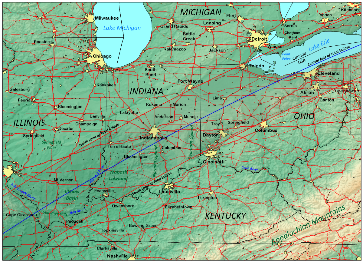
Along the portion of the track through Illinois, Indiana, Kentucky, and Ohio, there are small ups and downs in the topography (Figure 13), but no substantial elevation changes that would affect the cloud climatology. Past Toledo, the north side of the shadow track crosses Lake Erie and enters Canada, passing south of Lake St. Clair. The flat Canadian landscape has little influence on cloud cover but Lake St. Clair has some welcome benefits. In the United States, the south limit remains well away from the lake and cloud cover along that boundary is not influenced by the lake.
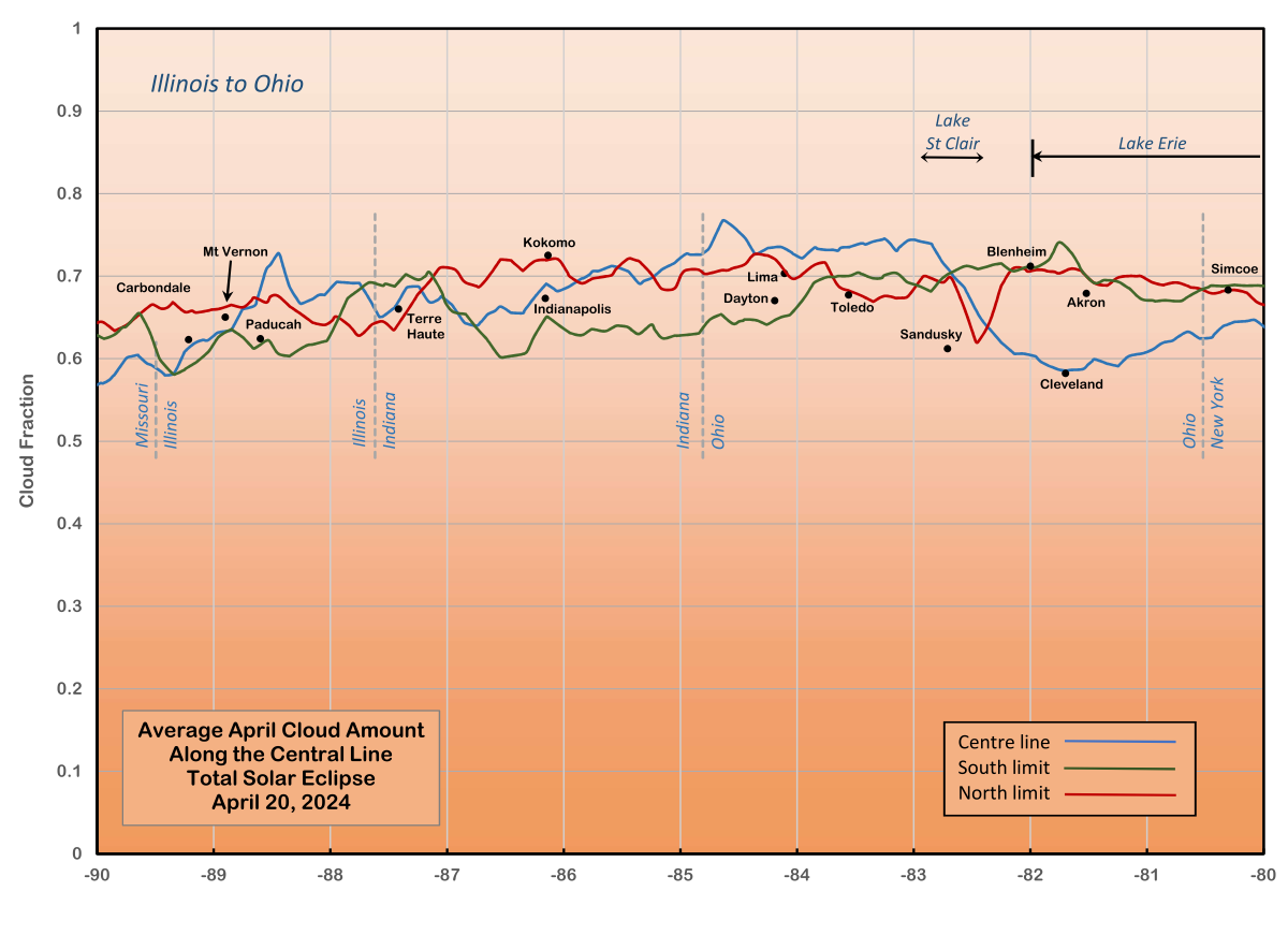
Figure 14 shows the satellite-based cloud amounts along the north and south limits as well as along the centreline. On the centreline, cloud amounts vary between 60 and 70 percent from Illinois to Lake Erie. The other traces show that there is no dominant side for either side of the track through the Midwest, except for a modest 5-8 percent lower cloudiness along the south limit from Owensboro, Kentucky, to Cincinnati, Ohio and a little beyond (Figure 14).
Just beyond Sandusky, Ohio, centre-line cloud in Figure 14 drops abruptly by more than 15 percent as the track reaches and crosses Lake Erie. The south-limit line, which passes 70 km (40 miles) to the south of the lake, doesn’t show this decline. The north-limit cloud trace shows a double minimum, a small, almost unnoticeable, broad dip just beyond Toledo where the track briefly passes over Lake Erie, and a much larger, sharper drop and recovery in Canada where the north limit passes south of Lake St. Clair. Figure 15s map confirms that these low-cloud refuges are created by the lakes, and that they are found above the lakes and for a short distance along and inland from the south shores. The south-side location indicates that lower cloud amounts tend to come on days with a northerly wind that extends the influence of the lake a short distance inland.
In April, the lake temperatures are likely only a degree or two above freezing (there is often ice on the lakes). On unsettled days, the afternoon often blossoms with cumulus and towering cumulus clouds and sometimes thunderstorms. Those clouds rely on heating from below, so the cold air over the lakes and the nearby lee shore suppresses the heating and the associated convective buildups and helps keep skies cloud free over the lake and for a few kilometres inland. This clearing is best seen in the satellite examples toward the end of this study.
North winds and unstable atmospheres are typically found on the backside of a departing low, behind a cold front. Satellite photos reveal that as the cloud along the cold front moves away to the east, the clearing that follows advances most rapidly along the south shore and more slowly inland. On light-wind days, the lakes may be completely surrounded by a band of clear skies while the land blossoms with convective clouds.
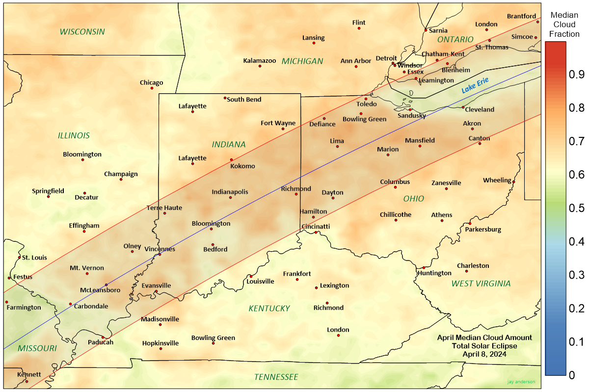
The main beneficiaries of this lake-induced suppression of cloud cover are communities that lie along the south and southwest shores of Lake Erie and south of Lake St. Clair in Canada. In particular, the city of Cleveland lies close to the spot with the lowest median cloud cover according to the satellite observations. In Canada, communities between Leamington and Blenheim will profit from being downwind of Lake St. Clair, though observations from this location will be very close to the north limit.
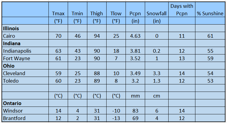
As a transitional month, April is no stranger to colder temperatures and a bit of snow. Once the track reaches Indiana, overnight lows below the freezing point are relatively common through the Midwest. Record lows reach to the -12°C (10°F) region and the average month has 2-8 cm (1 to 3 inches) of snow (Table 3). A wintery day before an eclipse will make for messy travel, but snowy days are uncommon—typically only 1 to 3 in the month. Sunshine statistics show show no particular trend from west to east, ranging in the 50 to 60 percent of the maximum possible. Though dated, these numbers are more encouraging than the cloud cover measurements from satellite. More will be said of this later.
Pennsylvania, Ontario, and New York
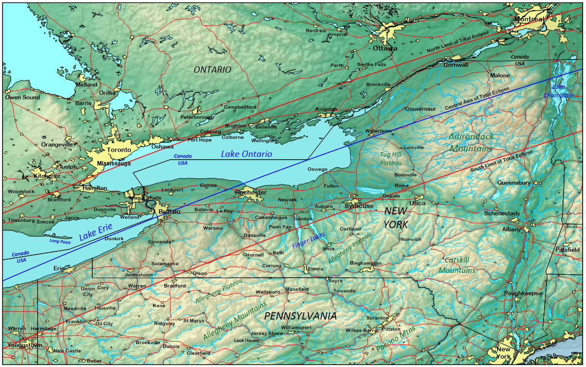
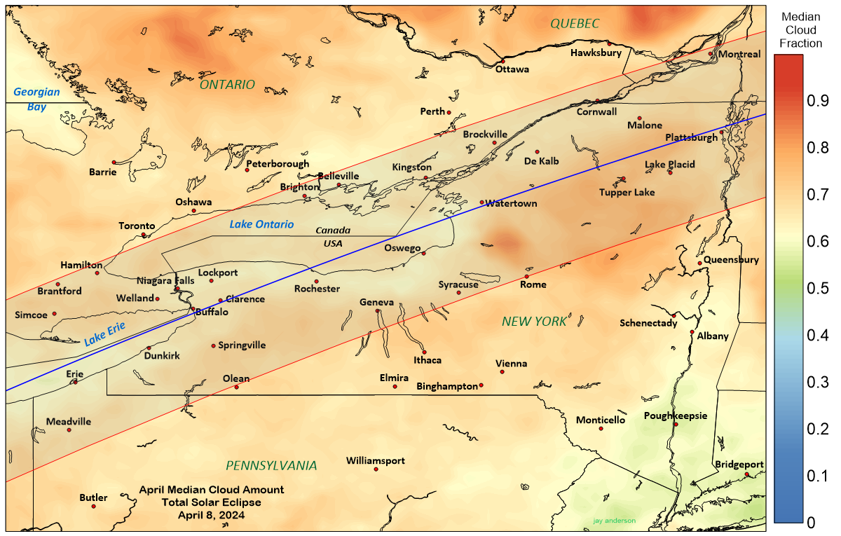
As the umbral shadow moves over Eastern Ontario and the Northeast States, it begins to cross the northern reaches of the Appalachian Mountains and terrain-induced cloud changes become significant. The north side of the track in Canada remains over lower terrain, first in crossing Lake Ontario, and then by moving down the valley of the St. Lawrence River. The south side, in contrast, passes over the Allegheny Plateau in Pennsylvania and western New York, and then over Tug Hill Plateau and the Adirondack Mountains in northeastern New York (Figure 16). Over Tug Hill, elevations reach 600 m above the lake level and over the Adirondacks, the south side of the track must climb above 1200 m. Generally speaking, rising terrain increases the amount of April cloudiness, while lower levels and the nearby presence of lakes brings lower cloud frequencies. These changes of elevation and circumstance are mirrored in the graph of cloud frequency along the eclipse path in Figure 17 and in the cloud map of Figure 18.
When we examine the three traces of cloudiness along the path in Figure 18, we find modest evidence of the mixed influences of topography and the nature of the underlying surface. Over Lake Erie, the centreline shows reduced cloud amounts but this tapers off toward the narrow end of the lake near Toronto and Buffalo (the station locations are plotted by longitude and so appear in unexpected positions along the graph). Lake Ontario’s influence is reflected in an 8 percent decline in cloudiness where the centre line approaches and crosses the shore at Rochester but the extent of the improvement in cloud statistics is better seen in the map of Figure 18, which shows that Lake Ontario is as effective as Lake Erie and Lake St. Clair in moderating cloudiness. In general, the south limit is cloudiest because it crosses a rougher and higher terrain and gets no benefit from the presence of the lakes.
The impact of the Adirondack Mountains is particularly noticeable in the centre and south-limit curves, with an increase of about 10 percent in the cloud cover. Tug Hill Plateau shows as a small bump in the central line trace, but its impact is muted because it lies between the eclipse midline and the south limit and none of the curves in the graph pass directly over it. Figure 18, however, shows that its effect on cloud cover is greater even than the Adirondacks, with average monthly amounts rising to 84 percent, the highest along this part of the eclipse track.
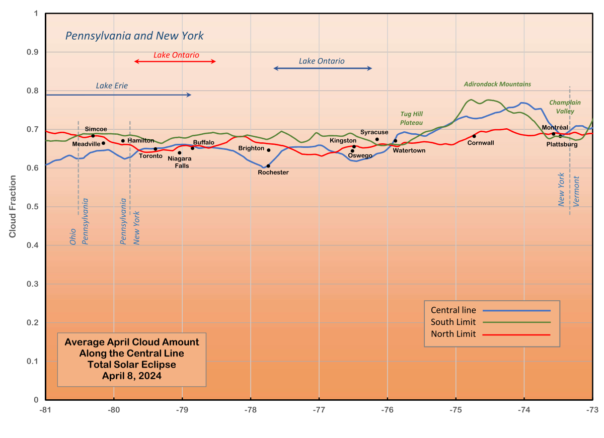
The upshot of all of this is that lower elevations and a position on the south side of the larger lakes will give a greater likelihood of sunshine on eclipse day. With some interruptions, there is a band of lower cloudiness along the south shore of Lake Erie as far east as Dunkirk, and along the south shore of Lake Ontario from Niagara Falls to Oswego and a little beyond. Rochester is particularly well located along the south shore of Lake Ontario with an median cloud amount of just over 60 percent in the month. Over Canada, there is little variation in cloud amount through this section of the eclipse track, though Figure 18 shows a small advantage to the Kingston area due mostly to the absence of adverse terrain.
After the shadow crosses the Adirondack Mountains, it drops into the Champlain Valley to move into Vermont. It’s a 700 metre drop, causing the cloudiness on the along the centre and south side of the shadow path to fall about 10 percent in response. On the north side of the track in Canada, the average cloud cover doesn’t change very much beyond Cornwall, remaining relatively low along the Saint Lawrence River valley and giving the region straddling the border from Kingston to Montréal a more promising forecast.
While the statistics identify regions of higher and lower springtime cloudiness from a 20-year average of satellite observations, the utility of such data is primarily for long-range planning. When we examine the satellite images individually to see how the weather systems behave, we find that clearing behind a weather system proceeds fairly regularly from west to east (no surprises there), but, as we’ve noted earlier, clearing along the lakefront proceeds more rapidly than elsewhere inland. This suggests a strategy for eclipse day if circumstances permit: move westward along the south shores of Lake Ontario and Lake Erie until skies clear if the day’s weather is affected by a passing low and cold front. Interstate 90 runs from Cleveland to Buffalo along Lake Erie, barely departing more than10 km from the water’s edge. Lake Ontario is not so well served, and smaller and more winding highways will have to suffice: Highway 104 runs from Rochester eastward, but leaves the waterfront and runs farther inland than seems comfortable.
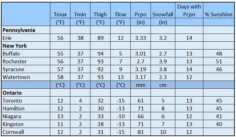
The northeastward path of the shadow brings the eclipse seeker into cooler climates. Average overnight lows through Ontario and New York flirt with the freezing point and nearly half the days of the month report precipitation of one form or another (Table 4). Snow days now become a possibility, though still only about 1 day in 10. The percent of maximum sunshine creeps downward with less than half the amount possible from sunrise to sunset. In such an environment, forecasts become more critical in the days leading up to the eclipse.
Vermont, New Hampshire, Quebec, and Maine to New Brunswick
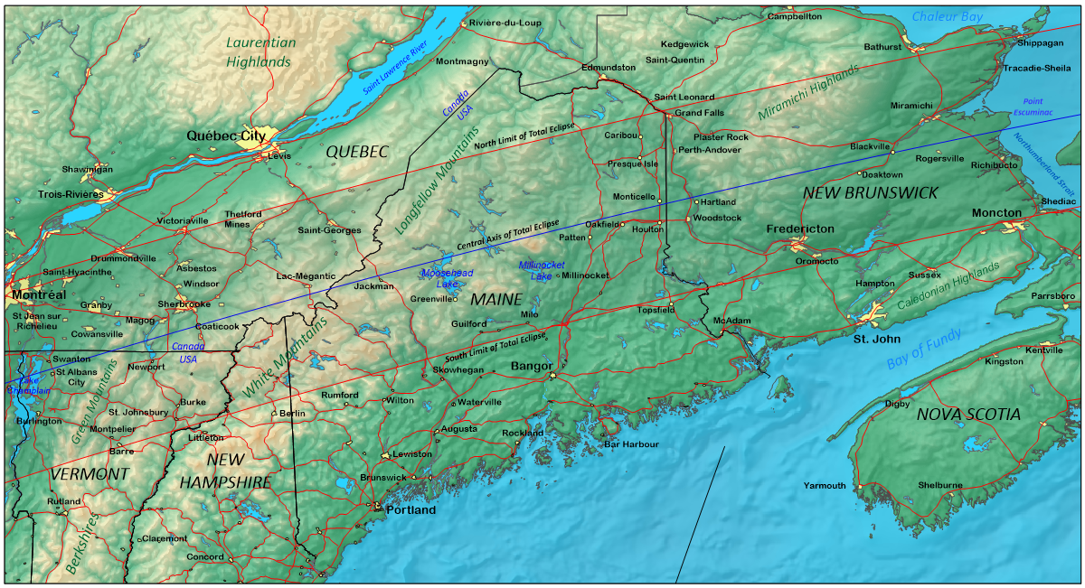
As the shadow path crosses into Vermont, cloud amounts climb in response to the gradual northward trend of the track that takes it ever deeper into the path of storms moving across the continent. The shadow also crosses the top end of the Appalachian Mountains in this region—the roughest terrain since Mexico. The south side of the eclipse path has the bumpiest route, negotiating a number of sub-ranges, the most prominent of which are the Green Mountains in Vermont and the White Mountains in New Hampshire, Maine, and a part of Québec (Figure 19). In contrast, the north side of the track passes over the flat plains of the St. Lawrence Valley south and east of Montréal before gaining a little elevation and roughness as it reaches the Maine border and the Longfellow Mountains (a branch of the White Mountains). The Appalachians begin to peter out in northeast Maine, leaving a rugged but lower-elevation landscape for the shadow as it moves into New Brunswick toward the Gulf of St Lawrence.
Along the centreline, the up-and-down character of the cloud pattern imitates the roughness of the terrain. Comparing the map in Figure 19 with the graph in Figure 20 and the map of Figure 21, it is apparent that the White and Longfellow Mountains generate higher amounts of cloud on their western sides . The drop in cloudiness over central Maine is a consequence of the downslope flow on the east side of the Longfellow Mountains, which dries the air and brings a 10 percent reduction in median cloudiness as the flow moves to lower elevations. Unfortunately, the mountains have another side effect: they create occasional wave clouds that spread across much of central and eastern Maine, sometimes reaching into New Brunswick. These clouds would not dissipate during the eclipse and may even thicken up, but they also have quasi-stationary open spots between the waves that might be exploited to view the eclipse.
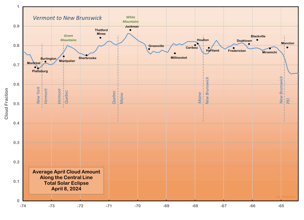
At first glance, it is difficult to be optimistic about eclipse-viewing prospects east of the Champlain Lakes. Along the Maine-Québec border, satellite-measured cloudiness reaches 90 percent across the White and Longfellow Mountains and barely falls below 75 percent over the rest of the path through eastern Maine and over New Brunswick (Figure 20). Weather prospects are consistently better at lower elevation, as seen by the tones in Figures 18 and 21 from Montréal to Granby over Québec.
Except for one place….
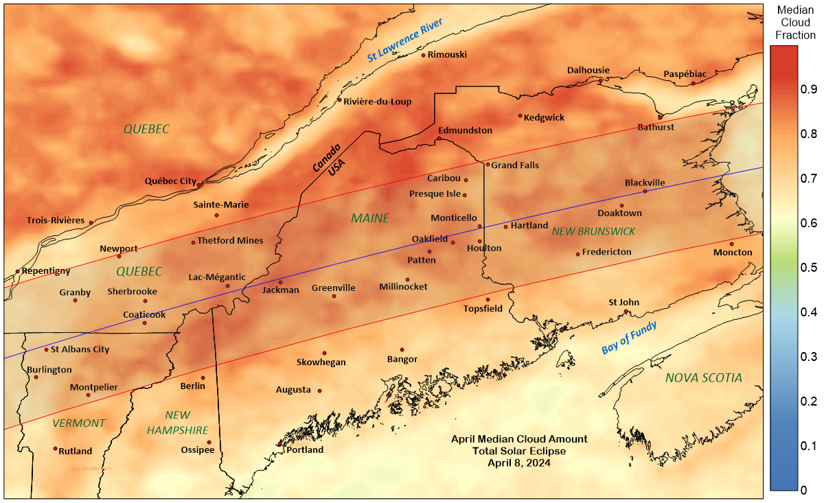
In Figure 20, the graph of centreline cloudiness shows an abrupt drop as the eclipse reaches the Northumberland Strait on the northeast coast of New Brunswick. More details are revealed in Figure 21, which shows that the largest part of this drop is over the Strait itself, extending only up to the land’s edge or a very short distance inland. This decline in over-water cloudiness is derived from those days each April when convective clouds form over the land when the Sun warms the ground but are unable to build above the cold waters of the Strait.
Examination of day-to-day satellite images argues for a location on the shores of the Gulf of Saint Lawrence. April is a month of extensive stratocumulus and cumulus clouds and the cold water of the Gulf is efficient at suppressing them. The advantage gained by settling along the Northumberland shore is not large—only about 15 percent—but it is the lowest level of cloudiness east of Lake Ontario. The Strait’s effect on the cloud cover is strongest where points of land project into the water such as at Point Escuminac or Richibucto Head (also known as Cap-Lumière).
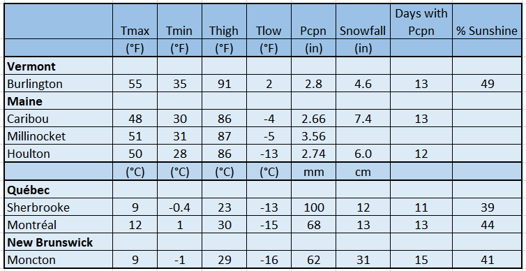
Once the lunar shadow moves past Ohio and Ontario, the promise of spring-like weather for the eclipse becomes less and less certain. From Cleveland to Montréal, climate observations show an average of 2-4 days of the month with snow. Average monthly accumulations are relatively small, generally 2.5 -10 cm (1-4 inches) through Ohio, New York, and Ontario growing to 10 – 18 cm (4-7 inches) in Québec, Vermont, and Maine (Table 5). Once into New Brunswick, however, average monthly snowfall increases to more than 30 cm (12 inches), and most years there will be snow on the ground on April 8, especially in Maine and New Brunswick.
Eclipse-day movement will be difficult In Maine and New Brunswick as both are notable for their wilderness character, and most of the roads run across the eclipse track instead of along it. The route from Bangor, Maine, to Fredericton, New Brunswick, only approximately follows the track, but will provide some room to roam. Limited mobility options will mean that eclipse-day movement decisions will have to rely on the forecasts.
While the satellite gives an idea of relative cloud cover from place to place, the sunshine statistics in Table 5 are more relevant for the actual probability of seeing the eclipse. Outline your strategy on the basis of the satellite images, but pick your spot with sunshine statistics in mind.
The Gulf of St. Lawrence and Newfoundland
After crossing Northumberland Strait, the moon’s shadow passes Prince Edward Island (PEI), just capturing the city of Summerside, and heads northeastward across the Gulf of St. Lawrence to bring Newfoundland its first eclipse since 1970. The low elevations on PEI (mostly under 40 m) and the Îles-de-la-Madeleine do not present any meteorological challenges. The umbral path does touch on the Cape Breton Highlands of Nova Scotia where elevations reach several hundred metres, but the rise in cloudiness there is mostly beyond the south limit of totality (Figure 22).
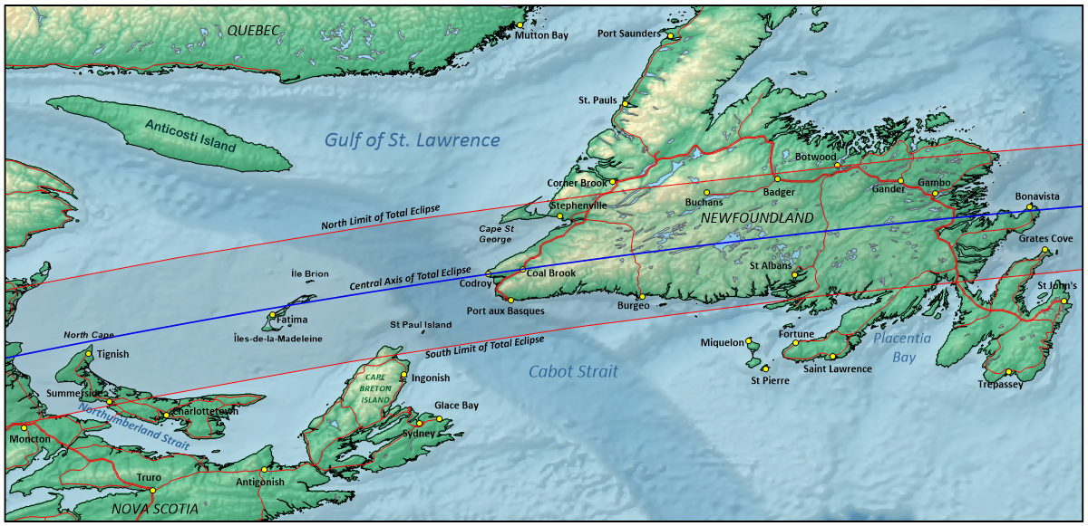
When the shadow reaches Newfoundland, terrain rises quickly from the shoreline as the north side of the track moves over the Annieopsquotch Mountains, east of Stephenville. The mountains are not particularly high, just under 700 m at their peak, but their influence on the cloud cover is apparent in Figure 23 and somewhat less so on the centreline graph of Figure 24 east of Codroy. After passing the mountains, the shadow settles onto the relatively flat terrain of Central Newfoundland, moving across a sparsely treed landscape of rolling hills until it reaches Bonavista Bay and heads out across the Atlantic. The south side of the umbral track has a smoother ride, delaying its arrival onto land until half-way across the island.
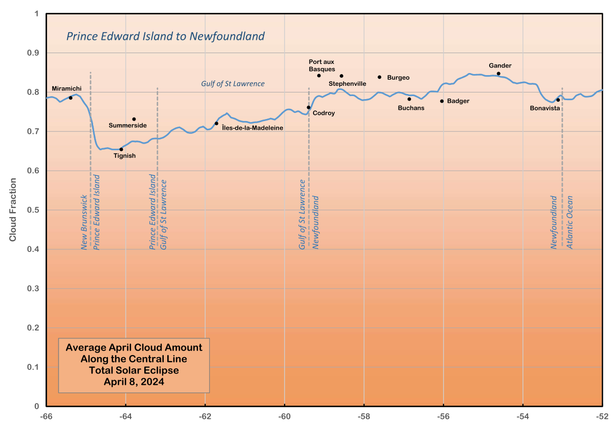
As we’ve noted earlier, cloud amounts fall abruptly to just under 65 percent (Figure 20) when the eclipse track moves off of the New Brunswick coast and out onto the waters of the Gulf of St. Lawrence. This sudden reduction is due almost entirely to the suppression of convection by the cold water of Northumberland Strait, as the average cloud amount pops up a small amount where the south side of the track crosses Prince Edward Island (Figure 24). This rise over PEI is not apparent in the centreline graph, but shows up vaguely in Figure 24. The north tip of PEI (North Cape) lies just south of the eclipse midline and this location, north of Tignish, is probably the best in Canada’s Maritime Provinces from which to view the eclipse. Close examination of Figure 24 indicates that the whole of the shoreline from North Cape to West Point benefits from the cold water of Northumberland Strait, with cloud amounts of just over 65 percent. These are a few percentage points better than the shoreline on the opposite side of the Strait, in New Brunswick.
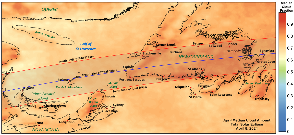
Beyond Prince Edward Island, the cloud cover climbs inexorably upward, from the minimum of 65 percent near Tignish to a discouraging 85 percent near Gander. There is a small upward bump as the shadow crosses the small rises in terrain in Newfoundland, and a modest decline as the shadow reaches Bonavista Bay before moving out to sea. Satellite images of Newfoundland show only one April 8 in the past 20 years where the whole island was clear, though there were several other years when partial openings or small holes in the cloud cover would have rewarded lucky observers.
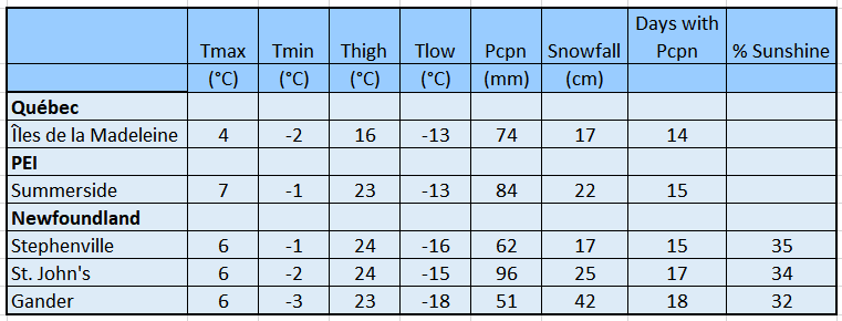
Not only are clear-sky prospects limited in Newfoundland, but winter is also entrenched and only beginning to give way to the spring warming. April’s morning lows are below the freezing point (Table 6) and precipitation is recorded on half the days of the month. Six to eight days of April get a snowfall to freshen the lingering winter snowpack and barely a third of the available daylight hours are sunny. The whole of the island is a tough place to catch a view of an eclipse. The most attractive part of eclipse watching in Newfoundland is probably Newfoundland itself.
Observations and Biases
When the MODIS cameras on the Aqua and Suomi satellites make their afternoon passage across the eclipse track (at around 1330 local time), they view the underlying terrain and cloud from an altitude of 700 km. The cameras have a ground resolution of between 250 and 1000 m depending on the waveband of observation. The highest resolution is reserved for the visible bandwidths.
Cloud cover estimates are made on the basis of a complex algorithm that incorporates radiance measurements from a subset of the 36 wavelengths bands observed from the satellite. That algorithm ends by assigning one of four values to each pixel: cloudy, probably cloudy, clear, and probably clear. The individual pixels are merged into larger blocks; those used in the maps on this site have a resolution of about 10 km. The cloud fraction (or percent of cloud amount) is simply the sum of cloudy and partly cloudy observations divided by the total number of observations.
It would seen that the view the Earth from 700 km would give the satellite pretty much a straight-down view of the clouds across the swath of terrain viewed from orbit. This not the case, however, as the curvature of the Earth dictates that views to either side of the satellite nadir are looking increasingly at the sides of clouds and not the top. This makes it appear that clouds are thicker toward the edges of the swath than in the middle, the same as happens for a human observer on the ground.
Satellites have other biases as well. You and I would identify clouds from orbit mostly by pattern recognition, but satellites see radiance values, often with different levels of sensitivity. Certain types of clouds show up strongly in some wavelength bands and less so in others, leading to a determination of cloudy or clear that depends on the particular algorithm used to assign decisions. Snow-covered surfaces fool visible wavelengths and cold ground in winter confuses infrared. One of the biggest challenges is to decide at what point a scene is “cloudy” when the clouds are translucent, especially at the cirrus level. In the end, there are several global measurements of cloud cover and all of them differ in some aspect. Ultimately, there is no such thing as a “correct” value for cloud amount.
Observations from the ground are worse and I have quit using them in these studies. You might want to gather some friends together and try estimating the amount of cloud cover in the sky on some day; you will not arrive at a consensus except for completely clear or completely cloudy days. In fact, at present, humans don’t make cloud observations in the U.S. and Canada any more. It’s done by machines that shine a series of laser pulses straight upward and wait for a reflection. If there’s a hole in the clouds, it’s clear, no matter what other cloud might be present in the surroundings. To compound the problem, the National Weather Service in the U.S. does not collect or process returns above 3700 m (12,000 ft.), and so detection is limited to low and some middle clouds and ignores the high mid clouds and cirrus types (cirrus clouds are defined to lie at 20,000 ft. or higher). A day of overcast mid and high cloud will be characterized as “clear.” As a result, some stations have a climatological record more than 90 percent clear skies, a record that would be hard to match in the sunniest places in the world.
Actual sunshine measurements can be more reliable, but those have not been conducted for many years in the United States; they were dropped at most sites beginning in 1994 and the last one in 2004. A few stations in Canada and many in Mexico are still taking observations. Figure 25 shows the trend of sunshine data along the eclipse track. There are no surprises here (except, perhaps, for North Little Rock), and the measurements show a general trend that follows the satellite data. More encouragingly, the sunshine amounts are more optimistic than the cloud data, a feature that you can probably accept as reasonably accurate. I wouldn’t suggest that the percent of possible sunshine is the actual probability of seeing the eclipse, but it is at least a good hint. Keep in mind that these are for the whole day and not for just the eclipse time.
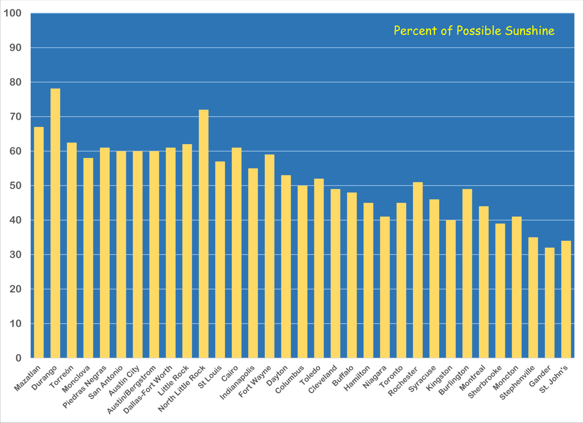
To give an example, at Moncton, New Brunswick, median April sunshine amounts to 41 percent of the sunrise-to-sunset hours according to the sunshine recorder. Compare this to the 79 percent cloudiness from the satellite and we are left with the conclusion that the satellite gives an overly pessimistic view of eclipse-day weather prospects. On the other hand, the measurement of cloud cover from the ground at Moncton’s airport gives a value of 82 percent average cloudiness for April. The satellite record (in this instance) is in close agreement with the ground observer, but at odds with the sunshine record.
So, who are we to believe? All observations have their biases. Sunshine recorders don’t “see” high-level, thin, cirrus clouds or the first and last minutes of the day. Automated ground-based cloud statistics are bothered with difficulties. Satellites must make a decision based on a set of wavelength radiances and a governing algorithm. In the end, the satellite data should be used to evaluate the relative advantages of one place over another, though we have to assume that whatever biases exist are common along the eclipse track (they aren’t but there is no easy way to fix the problem). Use the sunshine data (in Canada and Mexico) for an estimate of the true probability of seeing the event. At the very least, sunshine data should reassure the eclipse traveller that things are not as bad as they seem from orbit. By the time that eclipse day is only a week away, you will be looking at other information—satellite and model data.
To get a personal first-hand assessment of the cloudiness of your chosen eclipse site, take a look at the daily satellite data at NASA’s EOSDIS Worldview.
Eclipse-day planning
The 2024 total could be a meteorological challenge. This long-winded climate study is most useful for long-range planning, but becomes less and less helpful as eclipse day approaches. By late March, 2024, eclipse-day tactics should turn to the regular long- and short-range forecasts available from a number of agencies. On the day before the eclipse, numerical forecasts begin to lose some of their value as they are augmented by satellite and radar data and by reports from surface weather stations.
Satellites maintain a continuous watch across North America and the satellite of choice for this event is GOES East, located over the equator and streaming images at 5-minute intervals. There are few web sites that can do proper justice to the resolution of GOES E imagery, but I can recommend the one used by storm chasers: the College of DuPage (CoD) site at weather.cod.edu. At the College, you can look at an overview of the whole of the track across Mexico, the USA, and Canada, or you can zoom in to higher-resolution views of a particular state.
This eclipse comes in the middle of the day for the most part and so satellite images in visible wavelengths will be available for a few hours before the shadow reaches Mazatlán and for much of the day before reaching Bonavista. Visible-light images have the highest resolution, though a wider view with less zoom might prove more valuable if bigger weather systems have to be evaluated. If you are up all night trying to make a decision about an eclipse site, then you will have to make do with infrared satellite pictures, which are a bit harder to interpret. The CoD site gives you a choice of 16 different wavelength bands, plus a “true-color” composite for the daytime, but for nighttime use, you will probably want to choose one of the long-wave infrared (LWIR) bands. They come with garish colours, but because they are derived from thermal emission from the ground and clouds, they can be used in darkness.
Satellite photos are OK for what is happening now, but they are pretty limited for what will happen in the next day or two. For that information, we need to use computer forecasts (usually referred to as numerical forecasts or model forecasts). For single-point forecasts, there are a wealth of private and commercial choices, but I have grown to like the Spotweather site at spotwx.com. Spotwx will give you a model forecast for a single location, and will allow you to examine several different models to make some judgement about reliability of a prediction. Commercial sites usually only show you “their” model, as they don’t want to imply that there is some uncertainty in the future they foresee. In many cases, their model is actually the National Weather Service model with some fancy graphics attached.
Spotweather’s display is graphical in form, a very easy-to-follow display and compare but it doesn’t let you see what is happening in the neighbourhood. For that, we like to go back to the College of DuPage, as the same web address that gives satellite data also provides numerical forecasts. The forecast models are mostly the same as those provided by Spotweather, except that Spotweather also includes two Canadian models that are not available on CoD.
Models come in several forms, usually described by their resolution (how far the calculation points are separated), by their time frame (short-range or long-range), and by how often they are updated (1 to 12 hours). The differences between the models are much larger than these three elements, but those other differences are embedded in the code that runs the models, and so are not visible to you. The internal bits include such things as how cloud cover and precipitation are calculated, so you must expect some differences between models.
The main American models are the GFS (Global Forecast System) and the NAM (North American Model); the Canadian models are the GDPS (Global Deterministic Prediction System) and the RPDS (Regional DPS). From their names, you can see the extent of their forecast region. The global models make long-range forecasts, out to 15 days, while the regional models make forecasts for shorter time periods, usually 48 (RDPS) to 84 (NAM) hours. You will find other models on the CoD and Spotwx sites (the HRRR, the RAP, and the HRDPS) and you can look at them, but they are more specialized, usually used for thunderstorm forecasting (which might be needed). The models predict a large number of parameters, but you will be most interested in cloud cover and precipitation as the eclipse approaches.
A word of caution: models aren’t really very good until about a week ahead of an event, and improve steadily as the moment approaches. You will use the NAM and the RDPS for the two-three days ahead of the eclipse and the long-range models before. Once the models start to look like each other, with similar cloud patterns and precipitation amounts and when successive model runs keep the same forecast, you can begin to trust them. There will always be differences, but even that will tell you where things are uncertain and help you decide whether you might want to move to a spot where they all agree about good weather.
The global models work anywhere in the world and those forecasts that you get for your vacation spot in the tropics is probably derived from the GFS model, no matter who is hosting it. Spotwx will give you a forecast for “anywhere” just by inputting a latitude and longitude or clicking on a map, even in the middle of an ocean. Keep that in mind for your next eclipse.
When eclipse day arrives and the weather at your site is looking iffy, the local weather broadcast channel may be all that you need. For the most part, they concentrate on what’s happening now and what will happen in the next few hours. That may be all you need. In the end, preparation and mobility will be important.
Good luck on the 8th!
Historical satellite images
The following images will give some idea of the scope of the weather problems that you might encounter and offer some strategies for finding clear skies. These images are available after about 1:30 pm local time, probably too late to use for eclipse planning, but GOES East will provide the necessary images for last-minute moves.
Figure S1
Eclipse day in 2021 had a mixture of all of the elements that could cause problems with viewing an eclipse, but overall, skies were pretty decent, especially over the northeast. The main weather feature in Figure S1 is a large comma-shape storm centred over southern Indiana that kept skies cloudy from Missouri to central Pennsylvania. Clear skies hold sway across and south of the Great Lakes thanks to a large high-pressure system, but an old Atlantic storm brings a mixed bag of cloud and sunshine to the northeast, primarily affecting New Brunswick and Newfoundland.
Over Mexico, a patch of cirrus cloud carried by the sub-tropical jet stream brought variable conditions to Mazatlán and the central plateau. Except for a few places, the cloud would not have prevented a view of the eclipse, but more distant parts of the corona would probably be washed out. Over Texas, from San Antonio to Waco, morning stratocumulus gave way to scattered cumulus by eclipse time. Some patchy high cloud lingered in the Dallas area.
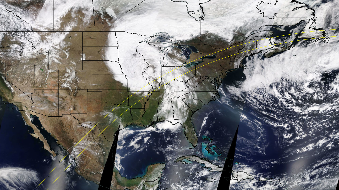
Figure S2
April 8, 2020, brought good weather to a large part of the eclipse track, from central Texas to Pennsylvania (Figure S2). In Mexico, high- and some mid-level cloud is spreading across the Pacific coast and into the interior, carried by the sub-tropical jet stream. The cloud is dense because of an off-shore disturbance that’s just visible in the lower left.
Unstable weather and the energy in the jet stream combine to promote the growth of thunderstorms along the U.S. border and through Texas, from Del Rio to Shreveport in northwest Louisiana . There is a considerable amount of higher-level cloud thrown off by these storms that could be avoided by moving to open skies in the neighbourhood while keeping an eye for new developments along the way. One of these storms generated a report of severe winds at a location east of the track.
Of more concern is the long tapered cloud just outside the eclipse track in Kentucky. This is a severe thunderstorm and the start of what became a day of severe weather that stretched from northern Arkansas into Ohio (Figure S1a). There were more than a dozen tornadoes, several of which formed under the eclipse track in Indiana and two under the track in Arkansas. In additions, the storms generated dozens of wind- and hail-damage reports. Eclipse seekers would have been secure on the north side of the centre line, but these events emphasize the need to keep an eye on severe weather forecasts for eclipse day.
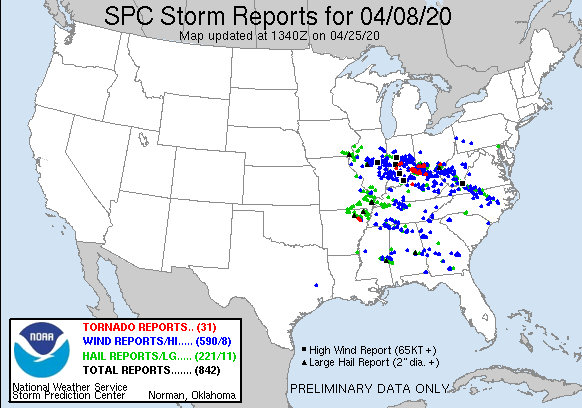
As the track reaches Lake Erie, it crosses an elongated band of cloud that stretches along the south shore of the lake. The white band is actually the remains of a thick morning fog that is just beginning to break up, turning into stratus and broken cumulus. Some parts of the band are likely to last through the day, but it is easy to escape by a small move westward or southward.
Over New York, cloud comes from a weak disturbance moving along a cold front that extends across the region into a deep low in the Atlantic south of Nova Scotia. Skies are clear over much of Maine under a high-pressure ridge, but New Brunswick is partly covered by broken stratocumulus that has been gradually dissipating since sunrise. Since the Aqua image was acquired at 13:30 local time, well before eclipse arrival time, there would probably be little cloud left by the time the sun is darkened. The stratocumulus does not extend across the Northumberland Strait shoreline, but does reform again over inland Prince Edward Island. Newfoundland is mostly cloudy in the south and central regions, but has a few breaks toward the northeast.
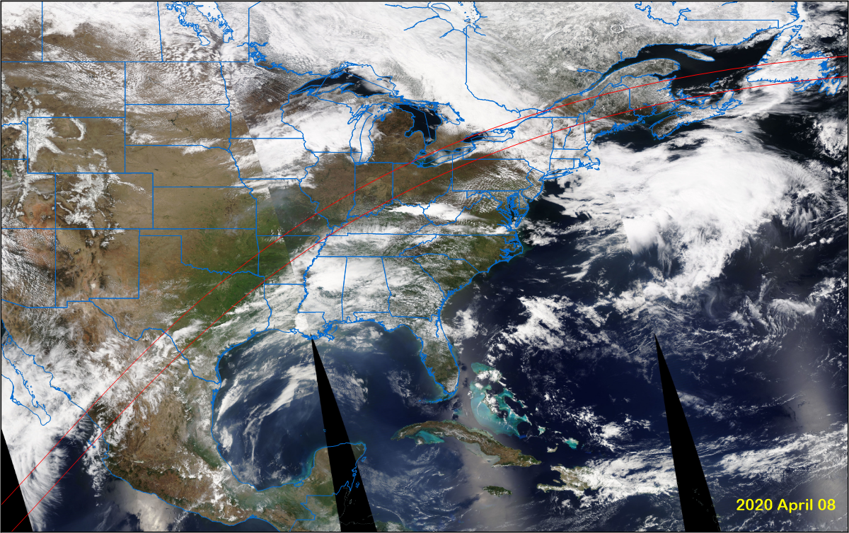
Figure S3
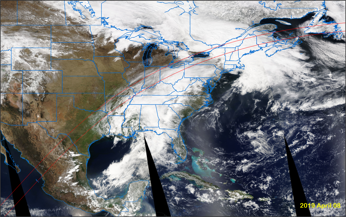
In Figure S3, Mexico is clear except for a few bits of cumulus cloud over the east slopes of the mountain ranges.
A large spring storm is curling around a low located near New Orleans; the back edge of this storm reaches as far west as Dallas; it is moving away from the eclipse track toward the southeast. From Dallas through Arkansas and into Missouri, the cloud is mostly thin cirrus with underlying cumulus clouds. The cumulus is small and recently formed, and would likely dissipate as the air cools ahead of the eclipse, but to be safe, observers should consider moving toward the north limit where clouds are thinner.
A cirrus veil overlies Illinois and Indiana, but Ohio and part of Pennsylvania is more solidly embedded in high and mid-level cloud. The cloud is moving slowly eastward, so the best bet through this region is to go toward the north limit, where the cirrus is less of an impedance.
Clear skies are available south of Lake Ontario (west of Rochester) and along the north shore in Canada from Toronto to Kingston thanks to a fortuitous position behind a cold front. Much of the cloud over southwest New York is moderately thin, allowing an unsatisfying but successful view of the eclipse.
Beyond Lake Ontario, the eclipse is likely hidden until the track reaches Prince Edward Island and the Gulf of St. Lawrence as it runs over a thick veil of cloud created by a low-pressure storm located near Cape Cod. Over Newfoundland, scattered to broken stratocumulus clouds would make the eclipse difficult, but not impossible with a small movement into a break in the clouds.
Figure S4
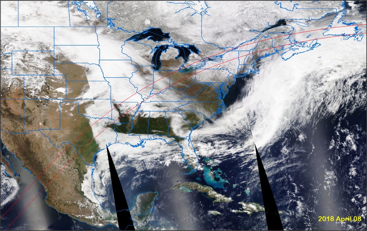
Figure S4 shows little of concern over much of Mexico and Texas, until the track passes Austin, Texas, where it runs into a thick overcast of fog and stratus that has moved northward from the Gulf of Mexico over the low-lying Mississippi floodplain. This cloud is burning off on its western edge, but very slowly. Humidities are very high, with dewpoints near 20°C (70°F).
From Arkansas to Indiana, the track crosses a broad band of cloud created by a moist southerly flow from the Gulf of Mexico. There are thin spots in the cloud here and there that will reward a few lucky observers with a fuzzy view of the eclipse. The track cross a region of clear skies in southwest Ohio but by the time it reaches the Pennsylvania border, colder air and a strong northwest flow has given rise to lines of stratocumulus, of which the thicker part will probably persist through the eclipse. Skies are clear from Erie to Cleveland in a narrow band along the south shore of Lake Erie because of the cool and stable air flowing off of the lake.
Unsettled and very cloudy weather persists as far as New Hampshire before breaking out into a semi-transparent cirrus veil over Maine and a bit of New Brunswick. It’s a brief respite, as the rest of the track past Newfoundland lies beneath a thick veil of cloud thrown up by a deep Atlantic low.
Figure S5
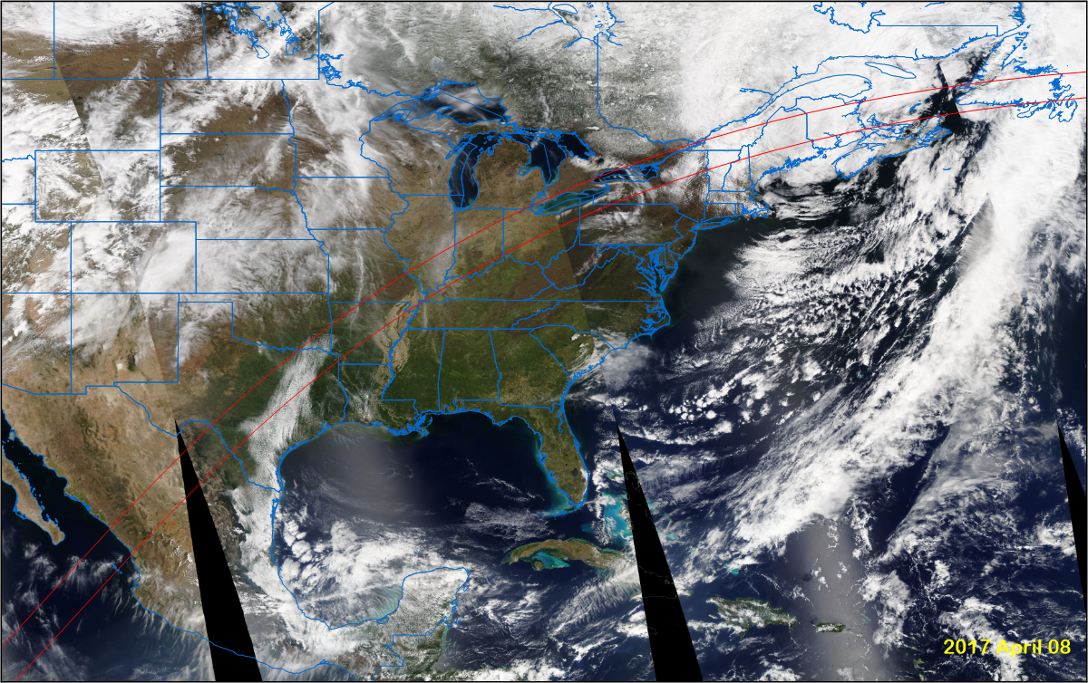
In Figure S5, Mexico and Texas along the border are relatively clear once again, but beyond San Antonio, the track runs across a broken field of cumulus and stratocumulus. This layer of low cloud, which is formed in the moist flow from the Gulf, pushes up against the Edwards Plateau near San Antonio, but is unable to penetrate farther to the west. It is gradually dissipating from the west but is probably too thick to dissipate during the eclipse. Eclipse-seekers from San Antonio to Austin and beyond could move to the north side of the track. The cloud may dissipate as the temperatures fall with the oncoming shadow, but most likely that will only happen along the west edge where the cloud is more scattered.
Past Oklahoma, it’s pretty much clear sailing to Rochester and Lake Ontario, at which point a small upper-air disturbance leaves a band of thin cirrus. The narrow white strip inland along the south shore of Lakes Erie and Ontario is actually snow on the ground; skies are clear in the area.
Over New York and for the rest of the track, watchers will have to deal with the cloud associated with a spring storm located centred over Québec’s Gaspe Peninsula. Over New York, Vermont and New Hampshire, it’s primarily stratocumulus wave clouds that will bring a mixture of cloud and sunny breaks. Wave clouds are stationary, and so openings remain in place and can be exploited beforehand to give a view to the sun. From Québec’s south shore and Maine, at least until Newfoundland, heavy cloud offers little encouragement. The southwest shore of Newfoundland near Codroy is promising because the cloud is thin and scattered, but past the middle of the island, the overcast returns.
Updated January 22, 2024
-Jay Anderson